REPRESENTATION LEARNING / WORLD MODELS

SADL: On the Demand-Supply Geometry
of Representation Collapse

Junhan Sun1 Yigui Feng2 Mingzhe Liu2 Haoyan Xu2 Lei Ye2
Ziqi Han2 Hanru Bai3 Yanzhao Zhang3 Hao Zhao2,4,† Guofeng Zhang1,5,†

1 Zhejiang University2 RoboParty Lab3 Alibaba Group4 AIR, Tsinghua University5 InSpatio

† Corresponding authors

An adaptive, one-sided Supply Regularizer
for stable representation learning.

Explore the research

SADL / VIDEO

SADL video

LeWM collapse rate

50%0%

LeWM encoder effective rank

14.552.7

INTACT control success

66.196.3%

Abstract

We propose SADL (Supply And Demand Loss), which keeps the original training objective and constrains the encoder directly when needed. SADL compares the representation differences that the projector output demands with the differences the encoder can retain and pass on to the projector, and adds a constraint on the encoder only when supply falls short of demand.

It works with different Demand Regularizers and introduces no auxiliary networks, additional trainable parameters, or architectural changes. We evaluate SADL on LeWorldModel (LeWM) and INTACT in single-task and jointly trained four-task control, and examine its generalization to image classification.

MOTIVATION

A well-constrained projector output
does not by itself prevent representation collapse.

Joint-Embedding Predictive Architectures (JEPAs) learn from images and video by predicting latent targets instead of reconstructing every pixel. An encoder maps inputs to a representation H, which a projector maps to an endpoint Z; existing Demand Regularizers typically constrain the geometry at Z.

In LeWM and INTACT, the encoder representation H is dominated by a component shared by all inputs from initialization. Batch normalization in the projector subtracts the batch mean. In training mode, adding the same vector to every row of H leaves Z unchanged, so neither the Demand Regularizer nor any loss computed from Z acts on the shared component of H.

The remaining variation grows mainly through the task gradient and concentrates in a few directions. The projector can remix and amplify existing variation to meet the Demand Regularizer's requirements, but cannot recover what H has lost.

On the shared direction, SADL supplies the nonzero gradient that the other losses lack; on the remaining directions, it lets the weaker ones grow faster.

Fraction of energy in sample variation

LeWM / EPOCH 1
Sample variation carried by H

+95.3 pp with SADL

Output regularizer only+ SADL
Baseline
3.3%
+ SADL
98.6%

Flash + SIGReg; fixed-probe medians across tasks and 10 training seeds. Gray: energy in the shared component.

METHOD

Demand and Supply Capacity

SADL reads a detached demand capacity q, measures the supply capacity k of H, and corrects H through a Supply Regularizer only when k < q.

The task loss and output regularizer remain in place. SADL adds a Supply Regularizer directly on the encoder representation.
01

Demand capacity

The demand capacity combines two terms from the detached endpoint: qreg increases as the Demand Regularizer is satisfied, while qexc measures the current sample variation at the endpoint. The demand capacity is the geometric mean of the two terms.
02

Supply capacity

SADL measures the supply capacity k as the weaker of the sample variation (excitation) in H and its transmission to Z. Hence k ≥ q requires both terms to reach q, so that even the smaller supply term meets the demand.

03

One-sided Supply Regularizer

We penalize insufficient supply capacity through a one-sided Supply Regularizer. It covers both excitation and transmission and is zero by construction whenever the supply capacity meets the demand capacity.

Training objective

L = Ltask+ λD D(Z)+ λS S(H, sg(Z))

The task loss and chosen output regularizer train as before. In the added term, sg stops gradients through Z, so the supply correction acts directly on H.

Adaptive demand

A constant demand must be re-tuned for each setting, whereas the adaptive q needs no tuning. Across five control and image settings, the adaptive q stays within seed variation of the best constant.

Demand and supply definitions

Demand from the output

q = √(qreg qexc)

qreg reads satisfaction of the output regularizer; qexc reads sample variation in Z.

Supply from the encoder

k = min{kexc, ktr}

kexc scores the energy and spread of sample differences in H. ktr measures linear association between H and Z through regularized canonical correlations.

S = [log(q + ε) − log(k + ε)]+2

ONE-SIDED CORRECTION

One-sided penalty

The penalty grows with the supply deficit. It is zero when supply reaches demand.

Illustration of the scalar penalty, not measured training data. Demand is detached during the encoder update.

S = [log(q + ε) − log(k + ε)]+2
PENALTY S0.598Correction active
No extra trainable parametersNo auxiliary networksOriginal architecture and inference

WORLD-MODEL CONTROL

Convergence and representation quality

We evaluate LeWM and INTACT on PushT, Cube, Reacher, and TwoRoom, reporting average control success across the four tasks.

Control success after one and two epochs

For both models and both backends, SADL after one epoch exceeds the baseline after two epochs. At epoch 2, INTACT + SADL reaches 96.3% mean success with either MATH or Flash.

Output regularizer only+ SADL
Exact values and experimental setup

Mean ± sample SD across 3 training seeds, using SIGReg. INTACT uses search-free Direct control; LeWM uses Pure-CEM. Within each pair, backends, update budgets, and evaluation are matched. The baseline retains the task loss and output regularizer, with no SADL term.

Four-task macro success (%)
ModelEncoder backendOutput regularizer only+ SADL

OUTPUT GEOMETRY

General adaptation across
Demand Regularizers

We test SADL with eight Demand Regularizers rather than assuming a single Gaussian target. After one epoch, all eight give INTACT over 92% search-free Direct success; seven reach 95.03–95.81%.

Epoch 1 control success95.58%

INTACT · 3 training seeds · four-task mean

PushTCubeReacherTwoRoom
1 / 8
SIGRegINTACT · Epoch 1 · Z · seed 0

Held-out endpoint representations · training seed 0 · 4,096 observations · PCA fitted jointly across tasks. Control success on the left averages three training seeds.

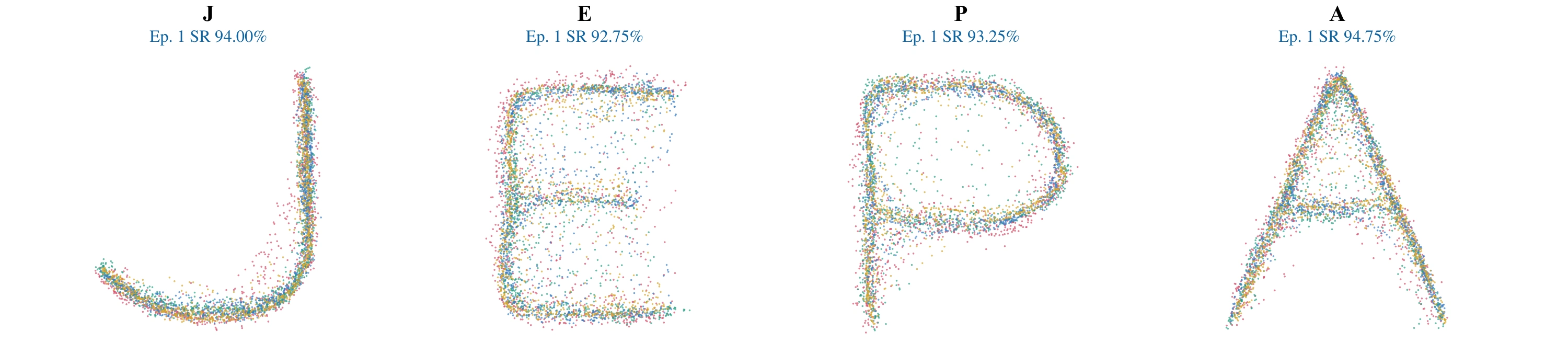
Actual learned representations. The eight regularizers show 3-D PCA views, with three-seed, four-task mean success rates. The separately trained 2-D glyph targets report single-seed success rates. Colors identify the four control tasks.
All output geometries

Student-t, GMM-Ring, Sphere shell, and VIC moments cover non-Gaussian or density-unspecified constraints. The separately trained glyph targets further illustrate adaptation to different endpoint geometries.

IMAGE REPRESENTATION LEARNING

Generalization to image tasks

Beyond control, we evaluate SADL on ImageNet-LT, Galaxy10, CIFAR-10, and Imagenette under matched budgets and Demand Regularizers.

SADL improves early learning across the four datasets. Imagenette gains 8.91 percentage points at epoch 20; the gap narrows to 0.44 points at epoch 800. On CIFAR-10, the main benefit is early in training, with little change at the final epoch.

BaselineSADL
Top: classification accuracy. Bottom: SADL minus its paired baseline, in percentage points. Mean ± SD over 3, 3, 10, and 7 seeds, respectively. CIFAR-10 uses a held-out ridge readout; the other datasets use online heads.
Imagenette · updates to baseline final accuracy23.2k 17.8k

23% fewer updates · median of 3 training seeds

ImageNet-LT · updates to 90% of baseline final accuracy34.8k 31.2k

10% fewer updates · median of 3 training seeds

Updates-to-target are measured in a separate three-seed comparison. Each target is defined by the baseline's final accuracy in that comparison.

Attention examples from the image experiments

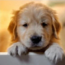
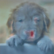
Input images and attention maps from VISReg and SADL + VISReg.

Input
Selected input from the ImageNet-LT attention experiment
VISRegSADL + VISReg
VISReg attention on the selected input SADL plus VISReg attention on the same input

CODE

Code coming soon.

Coming soon

BIBTEX

Citation

SADL: On the Demand-Supply Geometry of Representation Collapse

REPRESENTATION GEOMETRY

How the encoder preserves useful differences.

Learned glyph-shaped representations from the SADL paper
REPRESENTATION SPACE

Conceptual animation

Enlarged research figure